| Type | Class |
|---|---|
| Tags | programming, Project: Online Classes, computer science, compilers, mooc |
Compilers (Link)
- StanfordOnline: SOE.YCSCS1
A ten-week undergraduate course in compilers. The project of the course is to implement a compiler for Cool.
- Recommended readings
- Week 1: Introduction & the Cool Programming Language
- Week 2: Lexical Analysis & Finite Automata
- Week 3: Parsing & Top-Down Parsing
- Week 4: Bottom-Up Parsing I & II
- 07-01: Predictive Parsing
- 07-02: First Sets
- 07-03: Follow Sets
- 07-04: LL1 Parsing Tables
- 07-05: Bottom-Up Parsing
- 07-06: Shift-Reduce Parsing
- 08-01: Handles
- 08-02: Recognizing Handles
- 08-03: Recognizing Viable Prefixes
- 08-04: Valid Items
- 08-05: SLR Parsing
- 08-06: SLR Parsing Example
- 08-07: SLR Improvements
- 08-08: SLR Examples
- Week 5: Semantic Analysis and Type Checking
- Week 6: Cool Type Checking & Runtime Organization
- Week 7: Code Generation & Operational Semantics
- Week 8: Local Optimization & Global Optimization
- Week 9: Register Allocation & Garbage Collection
- Week 10: Java
Recommended readings
Although no textbook is required, there are recommendations provided for the interested student:
- Compilers: Principles, Techniques, and Tools, Second Edition (CPTT)
- Engineering a Compiler, Second Edition (EC)
- Modern Compiler Implementation in C (MCI), or the Java or ML version of the book
Suggested readings by topic:
- Lexical Analysis and Finite Automata
- CPTT: Sections 3.1, 3.3, 3.4, 3.6, 3.7, 3.8
- EC: Chapter 2 through Section 2.5.1 except for 2.4.4
- MCI: Chapter 2
- Parsing
- CPTT: Sections 4.1-4.6, 4.8.1, 4.8.2
- EC: Sections 3.1-3.5
- MCI: Chapter 3
- Semantic Analysis and Types
- CPTT: Sections 5.1-5.3 6.3, 6.5
- EC: Sections 4.1-4.4
- MCI: Chapters 4 and 5
- Runtime Systems and Code Generation
- CPTT: Sections 6.2, 7.1-7.4, 8.1-8.3, 8.6
- EC: Chapter 5, Sections 7.1-7.2
- MCI: Chapters 6, 7, and 14
- Optimization
- CPTT: Sections 8.5, 8.7, 9.1-9.4
- EC: Sections 8.1-8.4, 8.6, 9.1-9.3
- MCI: Chapter 10
- Advanced Topics: Register Allocation, Garbage Collection
- CPTT: Sections 7.5-7.6, Section 8.8
- EC: Sections 13.1-13.2, 13.4,
- MCI: Chapters 11 and 13
Week 1: Introduction & the Cool Programming Language
This week has 1:35:11 of lecture videos.
01-01: Introduction
A brief introduction: what is a compiler vs. interpreter, when and why were programming languages (starting with FORTRAN) developed.
01-02: Structure of a Compiler
Compilation works in five phases:
- Lexical analysis divides the program text into tokens.
- Parsing handles the grammar of the language--interpreting valid strings of tokens.
- Semantic analysis attempts to understand things like types--the meaning of the text.
- Optimization attempts to modify programs to use less time or space, for example.
- Code generation actually produces the machine code.
01-03: The Economy of Programming Languages
Programming languages and created in order to serve the different requirements of different application domains.
Most of the cost associated with using a new programming language is in training programmers, which leads to a few facts:
- New languages look like old languages, both because old languages might have good ideas, and because programmers are familiar with old languages, so require less training to become conversant in the new language.
- Popular languages can change only very slowly, because the cost of retraining a community of programmers is very high.
- New languages can be created and changed very 'cheaply', since they have few users.
02-01: Cool Overview
Cool is the Classroom Object Oriented Language. It is designed (by the instructor of this course, in fact) to be easy to implement.
This class will create a compiler from Cool to MIPS assembly language. There will be five programming assignments:
- Write a Cool program
- Lexical analysis
- Parsing
- Semantic analysis
- Code generation
Optimization will be touched on, as well.
A simple hello world program like the following is demonstrated:
class Main inherits IO {
   main(): SELF_TYPE {
        out_string("Hello, World.\n")
   };
};
02-02: Cool Example II
A program is demonstrated that takes an integer input and calculates the factorial, using both recursive and iterative techniques.
class Main inherits A2I {

    main() : Object {
        (new IO).out_string(i2a(fact(a2i((new IO).in_string()))).concat("\n"))
    };

    fact(i: Int): Int {
        let fact: Int <- 1 in {
            while (not (i = 0)) loop
                {
                    fact <- fact * i;
                    i <- i - 1;
                }
            pool;
            fact;
        }
    };
};
02-03: Cool Example III
Creating new classes is demonstrated. A list class that can print a string representation of itself is created.
class List inherits A2I {
    item: Object;
    next: List;

    init(i: Object, n: List): List {
        {
            item <- i;
            next <- n;
            self;
        };

    flatten(): String {
        let string: String <-
            case item of
                i: Int => i2a(i);
                s: String => s;
                o: Object => { abort(); ""; };
            esac
        in
            if (isvoid next) then
                string
            else
                string.concat(next.flatten())
            fi
    };
};

class Main inherits IO {

    main(): Object {
        let hello: String <- "Hello ",
            world: String <- "World!",
            i: Int <- 42,
            newline: String <- "\n",
            nil: List,
            list: List <-
                (new List).init(hello,
                    (new List).init(world,
                        (new List).init(42,
                            (new List).init(newline, nil))))
        in
            out_string(list.flatten())
    };
};
Week 2: Lexical Analysis & Finite Automata
This week has 2:22:30 of lecture videos.
03-01: Lexical Analysis
The goal of lexical analysis is to divide code up into its lexical units, called a lexeme, and to classify those units into the appropriate token class, such as identifiers, keywords, individual symbols, numbers, etc. The lexeme together with its token class make up a pair called a token.
03-02: Lexical Analysis Examples
In FORTRAN, whitespace is not significant. For example, VA R1 is the same as VAR1. As a result, DO 5 I = 1,25 begins a loop, while DO 5 I = 1.25 declares a variable--it is equivalient to DO5I = 1.25. In order to know whether the DO segment is a keyword for a loop or part of a variable name requires knowing what comes after. This is called lookahead.
In PL/I, keywords are not reserved. So something like this is valid:
IF ELSE THEN THEN ELSE; ELSE ELSE = THEN
Also in PL/I:
DECLARE(ARG1, ..., ARGN)
In this statement, DECLARE could, depending on context, be either a keyword or an array reference (if it is followed by =). Since there might have been any number of arguments (indices), it requires unlimited lookahead to determine which of the two is intended.
03-03: Regular Languages
Regular languages are used to specify the set of strings that belong to a token class. A regular language is usually described using regular expressions.
The language denoted by the regular expression `c' is a single-string language, namely \{``c"\}.
The language denoted by ε is the language consisting of the empty string, \{``"\}. Note that this is not the empty language!
The union of two regular languages is a regular language:
The concatenation of two regular languages is a regular language:
The iteration (i.e. the concatenation a finite number of times) of a regular language is a regular language:
This is called the Kleene closure or Kleene star.
The regular expressions over an alphabet Σ are the smallest set of expressions including the empty string, the single-character strings for each character in Σ, and the closure under union, concatenation, and iteration of these expressions.
03-04: Formal Languages
A meaning function maps expressions to the sets of strings that they denote.
This formalism is worthwhile because:
- It allows us to clearly distinguish syntax from semantics
- It allows us to consider notation as a separate issue
- Syntax does not map one-to-one to semantics: it is many-to-one.
Consider Roman vs. Arabic numerals. These have identical semantics, but very different syntax, and the latter is much more convenient for computation.
03-05: Lexical Specifications
- keywords: for example, 'if', 'then', 'else'
- integers: a non-empty string of digits, so:
- digit = '0', '1', ...
- integers = digit digit*
- or: integers = digit+
- identifier: a string of letters or digits, starting with a letter
- letter = 'a', 'b'..., 'A', ...
- or: letter = [a-zA-Z]
- identifier = letter (letter + digit)*
- whitespace: a non-empty sequence of blanks, newlines, and tabs
- whitespace = (' ', '\n', '\t')+
04-01: Lexical Specification
- Write regular expressions for each token class, e.g. identifier, whitespace.
- Construct R, matching all lexemes for all tokens (R = Keyword + Identifier + ..., a union of all the above regular expressions).
- Call the input x_1, ..., x_n, and for 1 \leq i \leq n check x_1...x_i \in L(R).
- If so, then that string is in some L(R_j) for some j.
- Then remove x_1...x_i from the input string and go to step 3.
What if there are two matching prefixes, e.g. there exists a j > i where both sequences up to x_i and x_j match? Then we take the maximal munch, which is the longest matching prefix.
What if multiple tokens match? For example, an otherwise valid identifier might also be a keyword. The usual rule is that keywords win, which is accomplished by a priority ordering, e.g. choose the regexp that was listed first.
What if no rule matches? Add a rule for errors that matches all strings not in the language, and put it last in priority.
There are good algorithms that accomplish this efficiently and require only a single pass over the input.
04-02: Finite Automata
A finite automaton consists of:
- An input alphabet Σ
- A finite set of states S
- A start state n
- A set of accepting states F ⊆ S
- A set of transitions: state ⟶input state
There is a graphical notation for finite automata:
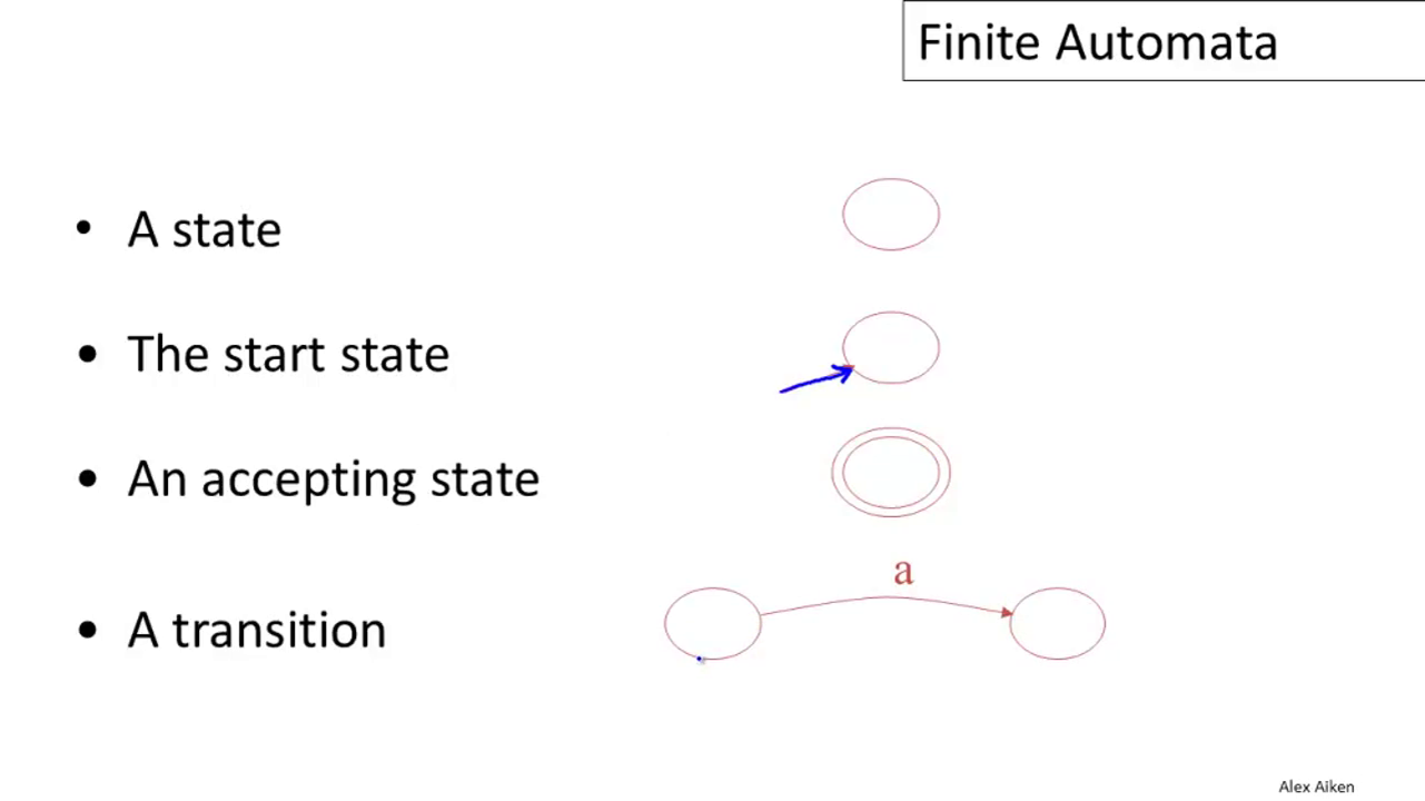
The language of a finite automaton is the set of all strings that it accepts.
A finite automaton can have another type of transition: ε-moves. These allow the machine to change state without consuming input.
A determininstic finite automaton (DFA):
- has only one transition per input per state
- no ε-moves
- takes exactly one path through the state graph per input
A non-deterministic finite automaton (NFA):
- may have multiple transitions per input per state
- may have ε-moves
- may take different paths through the graph for the same input
- accepts if any path terminates in an accepting state
Multiple transitions per input per state can be simulated by ε-moves, though it makes the automaton appear more complicated.
Both NFAs and DFAs recognize the same set of languages, the regular languages. DFAs are faster to execute, but NFAs are, in general, smaller than the equivalent DFA.
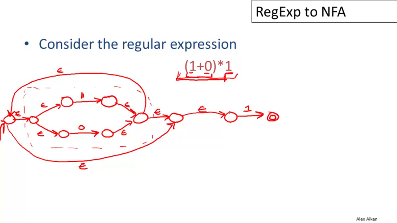
04-03: Regular Expressions into NFAs
For each regular expression M, we will define an equivalent NFA. This is done by composing the machines for each part of M using some simple rules. An example:
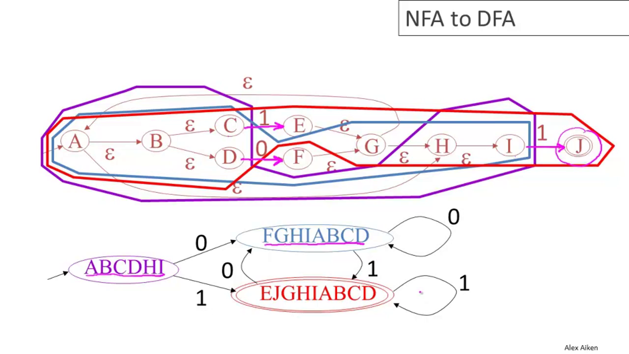
04-04: NFA to DFA
Call as the ε-closure of a state the set of all states that may be reached from it by any number of ε-moves, plus the state itself.
Given an NFA with states S, start state s, and final states F ⊆ S, define
and the ε-closure operation.
The states of the DFA will be all the nonempty subsets of S. The start state will be the ε-closure of s. The final states of the DFA will be
There will be a transition on the DFA X \rightarrow^a Y if
Converting the NFA from the last section to a DFA yields:
04-05: Implementing Finite Automata
A DFA can be implemented by a 2D table T:
- One dimension is states
- The other dimension is imput symbol
- For every transition from state i to state k on input a, define T[i, a] = k
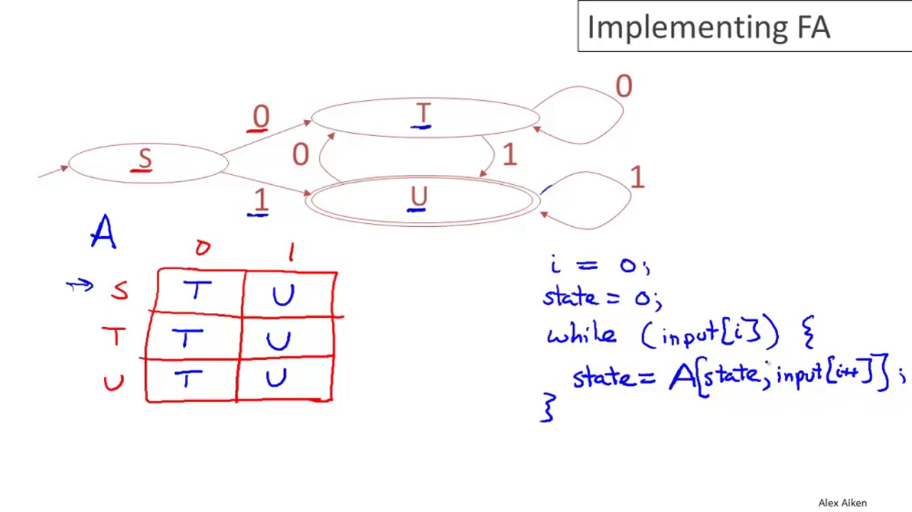
It can also be implemented as a one-dimensional table indexed on states and pointing to a table for the inputs. This would be more efficient if there are duplicated rows in T.
Alternatively, an NFA could be used directly, with a table containing sets of possible states.
Week 3: Parsing & Top-Down Parsing
05-01: Introduction to Parsing
Consider the language consisting of the set of all balanced parentheses:
This is not a regular language, and so cannot be expressed with regular expressions.
In general, a finite automaton can count things \mod k for some chosen k.
| Phase | Input | Output |
|---|---|---|
| Lexer | String of characters | String of tokens |
| Parser | String of tokens | Parse tree |
05-02: Context Free Grammars
A context-free grammar (CFG) consists of:
- a set of terminals, T
- a set of non-terminals, N
- a start symbol, s \in N
- a set of productions, \{x \rightarrow Y_1...Y_n \mid x \in N \land Y_i \in N \cup T \cup \{ \varepsilon \} \}
The productions may be viewed as a set of rules about substitutions that allow us to transform from a non-terminal start state to a state consisting only of terminals.
The terminals have no rules for replacment; they should be the tokens of the language.
Let G b a CFG with start symbol s. Then the language L(G) of G is:
Many grammars generate the same language. Tools may differ in how a grammar must be written.
05-03: Derivations
A derivation is a sequence of productions. A derivation can also be considered as a tree, where the children of a node are the elements to the right of the arrow in the grammar. This is the parse tree of the string.
A parse tree has terminals at the leaves, and non-terminals at the interior nodes.
An in-order traversal of the leaves is the original input.
In general, a parse tree may have many derivations. For parser implementation, we will be most interested in left-most derivations, in which the left-most children of the parse tree are resolved into terminals first, and right-most derivations, for the opposite case. These differ only on the order in which they are produced--the final parse tree is the same.
05-04: Ambiguity
A grammar is ambiguous if it has more than one parse tree for some string.
The ambiguity might be resolved by rewriting the grammar to eliminate the ambiguity (without changing the language).
Alternatively, accept the ambiguity, but define some disambiguating rules, such as precedence and associativity.
06-01: Error Handling
Three major kinds of error handling beavior:
- Panic mode
- Error productions
- Automatic local or global correction
The first two are in use today.
In panic mode, when an error is detected, it begins discarding tokens until it finds a synchronizing token, and then begins again. For examples, in (1 ++ 2) + 3, upon encountering the second + the compiler might begin skipping until it finds an integer, and continue from there.
Error productions specify known, common mistakes in the grammar. For example, writing 5 x instead of 5*x. This complicates the grammar, but allows alternate syntax for these cases.
Error correction attempts to find a 'nearby' program that does not have the error. You might try to find a program with a low edit distance, for example, that compiles. However, this is difficult to implement, slow, and may yield a program that compiles but behaves in the wrong way.
06-02: Abstract Syntax Trees
An abstract syntax tree (AST) is like a parse tree, but with some details ignored. For example, since the tree structure captures the nesting of the program, we don't need to keep track of the parentheses once parsing is complete.
06-03: Recursive Descent Parsing
Recursive descent is a top-down parsing algorithm. It constructs the parse tree from the top, and from left to right.
06-04: Recursive Descent Algorithm
For the grammar
A recursive-descent parser might be
bool term(TOKEN tok) { return *next++ == tok; }

bool E_1() { return T(); }
bool E_2() { return T() && term(PLUS) && E(); }

bool E() { TOKEN *save = next; return (next = save, E_1())
                                   || (next = save, E_2()); }

bool T_1() { return term(INT); }
bool T_2() { return term(INT) && term(TIMES) && T(); }
bool T_3() { return term(OPEN) && E() && term(CLOSE); }

bool T() { TOKEN *save = next; return (next = save, T_1())
                                   || (next = save, T_2())
                                   || (next = save, T_3()); }
06-04-1: Recursive Descent Limitations
The above parser will fail for input like int * int, because it will succeed at matching in T_1() and then conclude the program is done, leaving unconsumed input.
It fails as a whole because if a production for a non-terminal X succeeds, the parser has no way to go back and try an alternative production for X.
This is a limitation of the implementation, and not the overall strategy, though: general recursive-descent parsers support such "full" backtracking.
06-05: Left Recursion
Consider a production S \rightarrow S a.
bool S_1() { return S() && term(a); }
bool S() { return S_1(); }
This obviously contains an infinite recursion.
A left-recursive grammar has a non-terminal S S \rightarrow^+ S \alpha for some \alpha. Recursive-descent parsers do not work for left-recursive grammars.
Consider a grammar
This grammar is left-recursive. This language can be described by a right-recursive grammar:
A general algorithm for eliminating left-recursion can be found in Compilers: Principles, Techniques, and Tools, Second Edition. Compilers can and do eliminate left-recursion automatically.
Week 4: Bottom-Up Parsing I & II
07-01: Predictive Parsing
Predictive parsers are top-down, like recursive-descent, but they can 'predict' the correct production to use by looking at upcoming tokens (lookahead), without backtracking.
These parsers restrict the grammars. They accept LL(k) grammars. These are left-to-right grammars that use left-most derivation, and have k tokens of lookahead.
In LL(1) grammars, for each step, there is at most one choice of production.
Given the grammar
we can left-factor the grammar to remove common prefixes:
This grammar is converted to a parse table, and the unprocessed frontier of the parse is recorded in a stack. As items are matched using the parse table, they are pushed onto the stack, and matched terminals are popped off the stack. In the end, we should end up with an empty stack and all input consumed.
07-02: First Sets
Consider non-terminal A, production A \rightarrow \alpha, and token \mathrm t. Then T[A, t] = \alpha in two cases.
First, if \alpha \rightarrow^* \mathrm t \beta. In this case, \alpha can derive a \mathrm t in the first position, and we say that \mathrm t \in \mathrm{First}(\alpha).
Alternatively, if we have A \rightarrow \alpha and \alpha \rightarrow^* \varepsilon and S \rightarrow^* \beta A \mathrm t \delta, then we can eliminate A and proceed. In this case, we say that \mathrm t \in \mathrm{Follow}(A).
Formally, let us define
The algorithm to compute First is:
- \mathrm{First}(\mathrm t) = \{ \mathrm t \}, where \mathrm t is a terminal.
- \varepsilon \in \mathrm{First}(X)
- if X \rightarrow \varepsilon, or
- if X \rightarrow A_1...A_n and \varepsilon \in \mathrm{First}(A_i) for 1 \leq i \leq n
- \mathrm{First}(\alpha) \subseteq \mathrm{First}(X) if X \rightarrow A_1...A_n \alpha and \varepsilon \in \mathrm{First}(A_i) \textrm{ for } 1 \leq i \leq n
Consider the left-factored version of our favorite grammar:
Let us compute the first sets. For a given terminal, the first set is simply the set containing that terminal. For the other cases:
Since \varepsilon \notin \mathrm{First}(T), we know that
And for the other non-terminals:
07-03: Follow Sets
Formally define follow sets as:
Intuitively, we can see that if X \rightarrow A B then \mathrm{First}(B) \subseteq \mathrm{Follow}(A) and \mathrm{Follow}(X) \subseteq \mathrm{Follow}(B)
Also, if B \rightarrow^* \varepsilon, then \mathrm{Follow}(X) \subseteq \mathrm{Follow}(A).
If \mathrm S is the start symbol, then \$ \in \mathrm{Follow}(S).
The algorithm to compute follow sets goes:
- $ \in \mathrm{Follow}(S)
- \mathrm{First}(\beta) - \{ \varepsilon \} \subseteq \mathrm{Follow}(X) for each production A \rightarrow \alpha X \beta.
- \mathrm{Follow}(A) \subseteq \mathrm{Follow}(X) for each production A \rightarrow \alpha X \beta where \varepsilon \in \mathrm{First}(\beta).
Given the same grammar we worked with before, compute the follow sets. We can see these relations:
And therefore:
07-04: LL1 Parsing Tables
Not all grammars are LL(1). For example, a grammar is not LL(1) if it is:
- not left factored
- left recursive
- ambiguous
Most programming language CFGs are not LL(1).
07-05: Bottom-Up Parsing
Bottom-up parsing is more general than top-down parsing, but it is just as efficient. It is the preferred method used by most parsing tools.
Bottom-up parsers don't need left-factored grammars.
Bottom-up parsing reduces a string to the start symbol by inverting productions. If you read the reductions backward, you get a set of productions that amount to a right-most derivation.
07-06: Shift-Reduce Parsing
Bottom-up parsing uses only two kinds of moves: shift and reduce.
A shift reads one token of input. It pushes a terminal onto the stack.
A reduce applies an inverse production at the right end of the string. It pops symbols off the stack and pushes a non-terminal onto the stack.
08-01: Handles
It is not always correct to reduce as soon as reduction is possible.
A handle is a reduction that will allow further reductions back to the start symbol. Obviously, we only want to reduce at handles. Importantly, handles appear only at the top of the stack.
08-02: Recognizing Handles
There are no known efficient algorithms for finding handles, in general. However, there are good heuristics, which work on some CFGs reliably.
A viable prefix is one that, given an appropriate suffix, could be part of a handle. No parsing error has yet occurred.
For any grammar, the set of viable prefixes is a regular language.
08-03: Recognizing Viable Prefixes
We can build an NFA to recognize these.
08-04: Valid Items
08-05: SLR Parsing
Precedence declarations can resolve conflicts.
08-06: SLR Parsing Example
08-07: SLR Improvements
Most of the work of the DFA is repeated, because most of the stack does not change each time it is run. So, change the stack to hold pairs of (symbol, DFA state) to save time.
08-08: SLR Examples
Week 5: Semantic Analysis and Type Checking
09-01: Introduction to Semantic Analysis
Semantic analysis is the last "front end" phase.
In semantic analysis, coolc checks:
- All identifiers are declared
- Types
- Inheritance relationships
- Classes defined only once
- Methods in a class defined only once
- Reserved identifiers are not misused
09-02: Scope
The scope of an identifier is the portion of a program in which that identifier is accessible.
The same identifier can mean different things in different places due to different scopes.
An identifier may have restricted scope. Not all identifiers are global.
In a language with static scope, scope depends on the program text, not on runtime behavior. Most languages are of this type.
In a dynamically scoped language, like SNOBOL (or, formerly, LISP), scope cannot be determined until the program is run.
let x: Int <- 0 in
    {
        x;
        let x: Int <- 1 in
            x;
        x;
    }
In a statically-scoped language, an identifier's meaning is typically determined by the closest enclosing scope. In the above example, we can determine the value of the variable called x from the program text: the middle x is in the scope of the inner let, so it has value 1, while the other two are in the scope of the outer let, and have value 0.
In a dynamically-scope language, an identifier's meaning depends on the closest enclosing scope in the execution of the program, e.g. the closest binding on the call stack.
g(y) = let a <- 4 in f(3);
f(x) = a;
If the above example is in a dynamically-scoped language, then the value of a in f will be 4 when it is called from g.
In cool, class definitions are global. They are visible everywhere, and in particular can be used before they are defined. Similarly, attribute names are global within their class. Method names are more complex. They may be defined in a parent class, or overridden by a child class.
09-03: Symbol Tables
A symbol table is a data structure that tracks the current bindings of identifiers.
A simple way to implement a symbol table would be as a stack. When a new symbol comes into scope, push it onto the top of the stack. In order to resolve the meaning of a symbol, search from the top of the stack down, returning the first occurrence of the symbol. To remove the symbol, pop it off the stack. This stack-based symbol table will properly keep track of changing values in nested scopes.
This structure works well for let, which adds symbols one at a time, but not if multiple variables should be defined simultaneously in a new scope. To fix this, we can modify our structure to store entire scopes on the stack, rather than bare variables.
Since class names can be used before being defined, it is impossible to check class names using a symbol table, or in a single pass. Semantic analysis will require multiple passes.
09-04: Types
What is a type? It is a set of values along with operations supported on those values. In many languages, classes implement the notion of types. However, other languages may have other ways to implement types.
With regard to types, there are three kinds of programming languages:
- Statically typed languages do all or most type checking as part of compilation. (C, Java, Cool)
- Dynamically typed languages do all or most type checking as part of execution. (Scheme, Python)
- Untyped languages have no type checking. (machine language)
Terminology:
- Type Checking is the process of verifying fully typed programs.
- Type Inference is the process of filling in missing type information.
09-05: Type Checking
Type checking rules are simply logical inferences. For example: If e_1 has type Int and e_2 has type Int, then e_1 + e_2 has type Int.
Or, written in formal notation:
Use the turnstile symbol, \vdash to mean "it is provable that". We can write something like this:
To mean that given i is an integer literal, it can be proven that i has type Int. More usefully:
To apply this practically, we can show that 1+2 has type Int:
A type system is sound if everything provable within the system is true. There may be many sound inference rules, but not all are equally good. For example, all Ints are Objects in Cool, so any rule concluding an expression is an Int could also (less usefully) conclude that it is an object.
09-06: Type Environments
A type environment O is a function from ObjectIdentifiers to Types. It is used to tell the type checker the type of free variables which do not carry type information.
A useful bit of notation to support let providing a type to a new variable:
This notation indicates that we adjoin to O the rule that the type of x is T. Otherwise,
Within the let, then, we use O[T/x] as the type environment, and once we're back outside the let we return to O.
O is implemented in the type checker by the symbol table. This is a formalism representing the symbol table being passed down the AST.
09-07: Subtyping
Define a relation \leq on classes representing subtyping. This is a partial ordering where X \leq Y when X inherits from Y.
Consider an if expression:
if e_0 then e_1 else e_2 fi
The result could be either e_1 or e_2, so the type could be the type of either. Therefore, we can say, at best, that the type of the expression is the smallest supertype larger than the type of both e_1 and e_2.
Introduce a function lub(X,Y), the least upper bound of X and Y. Write:
In Cool, the least upper bound is the nearest common ancestor in the type inheritance tree.
09-08: Typing Methods
We will have a mapping M for method signatures:
This means that in class C there is a method f taking parameters of types T_1 through T_n and returning type T_{n+1}.
This M is provided to the type checker along with O. These are separate (in part) because in Cool there can be both methods and variables with the same name, which can be distinguished by context.
For some cases involving SELF_TYPE, we need to know the class in which an expression appears. So, the full type environment for Cool is:
- A mapping O giving types to object ids
- A mapping M giving types to methods
- The current class C
So sentences in Cool's type checker logic look like
NB: The rules and details here apply specifically to Cool, and will differ for different languages.
09-09: Implementing Type Checking
Just implement a recursive function that follows the inference rules.
Week 6: Cool Type Checking & Runtime Organization
10-01: Static vs. Dynamic Typing
The static type of a variable is the type predicted at compile time by the type inferencer. The dynamic type of a variable is the type it actually has at runtime. So, a simple soundess rule is that for all expressions E, dynamic_type(E) = static_type(e).
However, the actual situation is more complex. Consider:
class A { ... }
class B inherits A { ... }
class Main {
    x: A <- new A;
    ...
    x <- new B;
    ...
}
In the first line of Main, x's static and dynamic types match: A. Later, though, x has dynamic type B, a subtype of A. For Cool, then, the soundness theorem is a little more complex:
Subclasses must support all attributes and methods of parent classes, so subclasses can only add attributes or methods. Further, overridden methods must have the same type.
10-02: Self Type
The SELF_TYPE keyword allows methods to return whatever type self has, so it is useful when subclassing. Without this, methods that return self will fail typechecking in subclasses.
10-03: Self Type Operations
Write as \mathrm{SELF\_TYPE}_C an occurrence of SELF_TYPE in the body of a class C. Then,
More rules:
10-04: Self Type Usage
SELF_TYPE cannot necessarily be used where other types could be used, because it is not a type class. In particular, it cannot be assigned as the type of a formal parameter in a method.
10-05: Self Type Checking
By extending the definitions of lub and \leq as above, there will generally be little modification needed for the type rules to work with SELF_TYPE.
10-06: Error Recovery
When type checking, if the correct type cannot be determined, we could assign type Object to the expression. This will leade to a cascade or errors as the type is propagated up the AST.
We could introduce a new type, No_type, defined for type-checking as No_type <= C for all types C, and producing a No_type result for all operations. This is a realistic solution for a real compiler, but a little more trouble to implement, since the class hierarchy will no longer be a tree.
11-01: Runtime Organization
So far, we've covered the front-end phases of the compiler, which are concerned with the language definition: parsing the program and ensuring it is valid. Next, we will cover the back-end phases, including code generation and optimization.
When a program is initially invoked:
- the OS allocates space for the program
- the code is loaded into that space
- the OS jumps to the program's entry point
The memory allocated to the program is segmented into several (perhaps non-contiguous) sections, including sections for code and data.
11-02: Activations
There are two goals of code generation: correctness and speed.
Two assumptions:
- Execution is sequential; the control flow of a program is well-defined.
- When a procedure is called, control returns to the point immediately after the call.
These assumptions need not be valid. A concurrent language will violate the first, and language constructs like exceptions will violate the second. But for the purposes of the class, these will be held true.
Define:
- an invocation of procedure
Pis an activation ofP - the lifetime of an activation of
Pis all the steps to executeP, including the steps in procedures called byP - the lifetime of a variable
xis the portion of execution in whichxis defined- note that lifetime is a dynamic (run-time) concept; scope is a static concept
When P calls Q, then Q returns before P does. Therefore the lifetimes of procedure activations are nested, and can be depicted as a tree.
The activation tree depends on run-time behavior, and may vary depending on input.
Since activations are nested, they may be tracked with a stack.
11-03: Activation Records
The information needed to manage one procedure activation is call an activation record (AR) or frame.
If a procedure F calls G, then G's AR contains info about both F and G. The AR contains information needed to complete execution of the procedure, and resume execution of the parent procedure.
11-04: Globals and Heap
A variable is global if all refernces to it point to the same object. In this case, it cannot be stored in an activation record, as a function argument might be. Instead, a global will be assigned a fixed address by the compiler; call this statically allocated.
Any other value that must outlive the procedure that creates it must also be stored outside the activation record. Such values are typically stored on the heap.
The memory space of a program is typically divided into:
- the code area
- often of fixed size and read-only
- the static area, for data with fixed addresses
- fixed size, may be writable
- the stack
- the heap
Both the heap and the stack grow during runtime. Typically, they start at opposite ends of memory and grow toward each other.
11-05: Alignment
Data is word aligned in memory if it begins at a word boundary. There are often performance penalties if data is not word aligned, or even absolute restrictions against it. For this reason, it is important to ensure that data is aligned in the manner preferred by the machine.
11-06: Stack Machines
A stack machine has only a stack for storage.
An instruction r = F(a_1, ..., a_n):
- pops
noperands from the stack - computes the operation
Fusing the operands - pushes the result
ronto the stack
Importantly, the contents of the stack prior to that instruction remain unchanged.
Java uses a stack machine model.
There is a benefit to register machines: they tend to be faster. A compromise is possible. An n-register stack machine is one that, conceptually, keeps the top n locations of the stack in registers. In a 1-register stack machine, the register is called the accumulator.
Week 7: Code Generation & Operational Semantics
12-01: Introduction to Code Generation
The MIPS architecture is the prototypical RISC architecture. Most operations use registers for operands and results. There are 32 general purpose registers, of 32 bits each.
MIPS instructions:
lw reg_1 offset(reg_2)- load a 32-bit word from address
reg_2 + offsetintoreg_1
- load a 32-bit word from address
add reg_1 reg_2 reg_3reg_1 <- reg_2 + reg_3
sw reg_1 offset(reg_2)- store a 32-bit word in
reg_1at addressreg_2 + offset
- store a 32-bit word in
addiu reg_1 reg_2 immreg_1 <- reg_2 + imm- "u" means overflow is not checked (unsigned)
li reg immreg <- imm
A program to implement 7 + 5 on MIPS:
li    $a0 7
sw    $a0 0($sp)
addiu $sp $sp -4
li    $a0 5
lw    $t1 4($sp)
add   $a0 $ao $t1
addiu $sp $sp 4
12-02: Code Generation I
Code generation for the stack machine is a recursive endeavour. To support it, we must satisfy two invariants:
- after the code for an expression has run, the result of that expression is in the accumulator
- after the code has run, the stack is in the same state it was before the code was run
We'll use a simple language with obvious semantics for the following examples.
For evaluating a constant, define:
cgen(i) = li $a0 i
This loads the constant into the accumulator, leaving the stack untouched. Trivial! Something slightly more complex:
cgen(e_1 + e_2) =
  cgen(e_1)
  sw    $a0 0($sp)
  addiu $sp $sp -4
  cgen(e_2)
  lw    $t1 4($sp)
  add   $a0 $t1 $ao
  addiu $sp $sp 4
Since each cgen step obeys the invariants, we can be confident in the behavior of this code.
New MIPS instructions:
beq reg_1 reg_2 label- branch to
labelifreg_1 == reg_2
- branch to
b label- unconditional jump to
label
- unconditional jump to
cgen(if e_1 = e_2 then e_3 else e_4) =
  cgen(e_1)
  sw    $a0 0($sp)
  addiu $sp $sp -4
  cgen(e_2)
  lw    $t1 4($sp)
  addiu $sp $sp 4
  beq   $a0 $t1 true_branch
false_branch:
  cgen(e_4)
  b     end_if
true_branch:
  cgen(e_3)
end_if:
12-03: Code Generation II
cgen(f(e_1, ..., e_n)) =
  sw    $fp 0($sp)
  addiu $sp $sp -4
  cgen(e_n)
  sw    $a0 0($sp)
  addiu $sp $sp -4
  ...
  cgen(e_1)
  sw    $a0 0($sp)
  addiu $sp $sp -4
  jal   f_entry
This is the caller's side of the function call.
New instruction:
jr reg- jump to address in register
reg
- jump to address in register
cgen(def f(x_1, ..., x_n) = e) =
  f_entry:
    move  $fp $sp
    sw    $ra 0($sp)
    addiu $sp $sp -4
    cgen(e)
    lw    $ra 4($sp)
    addiu $sp $sp z
    lw    $fp 0($sp)
    jr    $ra
The size of the activation record is z = 4*n + 8, which is known at compile time--that's a static value.
Note that the callee pops the return address, arguments, and fp off the stack.
12-04: Code Generation Example
A sample program:
def sumto(x) = if x = 0 then 0 else x + sumto(x-1)
sumto_entry:
  move  $fp $sp
  sw    $ra 0($sp)
  addiu $sp $sp -4
  lw    $a0 4($sp)
  sw    $a0 0($sp)
  addiu $sp $sp -4
  li    $a0 0
  lw    $t1 4($sp)
  addiu $sp $sp 4
  beq   $a0 $t1 true1
false1:
  lw    $a0 4($fp)
  sw    $ao 0($sp)
  addiu $sp $sp -4
  sw    $fp 0($sp)
  addiu $sp $sp -4
  lw    $a0 4($fp)
  sw    $a0 0($sp)
  addiu $sp $sp -4
  li    $a0 1
  lw    $t1 4($sp)
  sub   $a0 $t1 $a0
  addiu $sp $sp 4
  sw    $a0 0($sp)
  addiu $sp $sp -4
  jal   sumto_entry
  lw    $t1 4($sp)
  add   $a0 $t1 $a0
  addiu $sp $sp 4
  b     endif1
true1:
  li    $a0 0
endif1:
  lw    $ra 4($sp)
  addiu $sp $sp 12
  lw    $fp 0($sp)
  jr    $ra
This is fairly inefficient code, since we have generated it using the very simple stack machine model. Optimizations are possible!
12-05: Temporaries
We can compute the (maximum) number of temporary variables needed to compute an activation in advance. Then, we can add space for those to the activation record.
Essentially, this will allow the stack arithmetic previously needed to be computed at compile time. Then the values can be saved and loaded from static offsets.
Consider the code for cgen(e_1 + e_2) we had before:
cgen(e_1)
sw    $a0 0($sp)
addiu $sp $sp -4
cgen(e_2)
lw    $t1 4($sp)
add   $a0 $t1 $ao
addiu $sp $sp 4
Using temporaries in the AR, we can instead have:
cgen(e_1, nt)
sw  $a0 nt($fp)
cgen(e_2, nt+4)
lw  $t1 nt($fp)
add $a0 $t1 $a0
Here, nt is the offset into the frame of the first available temporary slot.
12-06: Object Layout
Take the following sample objects:
class A {
  a: Int <- 0;
  d: Int <- 1;
  f(): Int { a <- a + d };
};

Class B inherits A {
  b: Int <- 2;
  f(): Int { a };
  g(): Int { a <- a - b };
};

class C inherits A {
  c: Int <- 3;
  h(): Int { a <- a * c };
};
- Objects are laid out in contiguous memory
- Each attribute is stored at a fixed offset in the object
- The offset of the attribute is the same in every object of that class
- The offset of the attribute is the same in all subclasses of the class
- When a method is invoked, the object is
selfand the fields are the object's attributes
In Cool, the first 3 words of an object contain header information:
- Class Tag
- An integer that identifies the class of the object
- Object Size
- An integer, the size of the object in words
- Dispatch Pointer
- A pointer to a table of methods
Following this are the attributes.
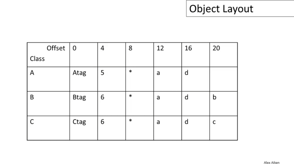
Now, consider dynamic dispatch. The situation for the dispatch table is similar to that for attributes.
- Each class has a fixed set of methods, including inherited methods
- The dispatch table contains pointers to the entry point of each method
- A method
flives at a fixed offset in the dispatch table for a class and all of its subclasses
13-01: Semantics Overview
Three ways of describing the behavior of a program:
- Operational semantics describe program evaluation (on an abstract machine) via execution rules
- Denotational semantics describe the program's meaning as a mathematical function
- Axiomatic semantics describe program behavior via logical formulae
- e.g. "if execution begins in a state satisfying X, then it ends in a state satisfying Y", where X and Y are formulas in some logic
- can be used as a foundation of automated program analysis systems
13-02: Operational Semantics
Let us introduce a notation:
Undersand this as "In the given context, expression e evaluates to value v.
For example:
13-03: Cool Semantics I
13-04: Cool Semantics II
Week 8: Local Optimization & Global Optimization
14-01: Intermediate Code
A compiler might have one or several intermediate languages that abstract away some details from the target language (i.e. details of the target machine). This can simplify writing a compiler with multiple targets, enable easier optimization (e.g. by introducing a concept of registers, which do not exist in Cool), or provide other benefits.
The IL of interest in this course, used for Cool, is like an abstract assembly language with an unlimited number of registers. It is a three-address code, in which each instruction contains at most three addresses: the target into which to store a result, and either a unary or binary operation to compute.
14-02: Optimization Overview
A basic block is a maximal sequence of instructions with no labels, except at the first instruction, and no jumps, except at the last instruction. This means that control flow in a basic block is totally predictable.
14-03: Local Optimization
Local optimization optimizes a single basic block.
14-04: Peephole Optimization
Optimization on a sequence of contiguous assembly instructions.
15-01: Dataflow Analysis
15-02: Constant Propagation
15-03: Analysis of Loops
Loops have (at least) two entry points: the initial entry point, and returning from the end of the loop. This creates a recursive problem for determining the value of variables. Solution: set the value to \bot, then work your way through the control flow graph until you get back the the start of the loop, and see if it is consistent.
15-04: Orderings
For constants c, we have:
Constants are equal to themselves, but incomparable to other constants. This is a partial ordering.
Write as lub the least upper bound of a set of elements. Then the rule for constant propagation is:
15-05: Liveness Analysis
A variable assignment is live if that variable may be accessed later, and if it is not overwritten before that access. Working backward along the control flow graph, then, we can compute the liveness of variables. Take:
Then we can define the liveness rule similarly to the constant propagation rule:
Week 9: Register Allocation & Garbage Collection
16-01: Register Allocation
Construct a graph, called a register interference graph (RIG), where the nodes are temporaries in the IR, and an edge exists between two nodes if the corresponding temporaries are ever live simultaneously in the program.
16-02: Graph Coloring
A coloring of a graph is an assignment of colors to nodes, such that nodes connected by an edge have distinct colors.
A graph is k-colorable if it has a coloring with k colors.
For our purposes, colors correspond to machine registers. If a RIG is k-colorable, then it needs at most k machine registers.
An algorithm for coloring a RIG:
- Pick a node
twith strictly fewer thankneighbors - Remove
t(and its edges) - If the resulting sub-graph is k-colorable, then so is the original
Iterate until the graph is empty (of course, it may be that the process will terminate without all nodes being removed). Now, build the graph back up, assigning valid colors to the nodes one at a time, as they are added to the graph. We are guaranteed to be able to do this, and so can construct a complete coloring.
16-03: Spilling
If we cannot find a k-coloring, then some values will have to be stored in memory (spilled into memory).
So, pick a candidate f for spilling, and remove it from the graph. If we are fortunate, then the remaining subgraph can be colored such that the neighbors of f use fewer than k colors. Then we can add f back in with a free color, and continue--f did not actually need to be stored in memory. This technique is optimistic coloring.
If optimistic coloring fails, we must allocate memory for f. Typically, we will store it in the current stack frame. If we call that address fa, then we must modify the code, so that before each operation that reads f, we have f:= load fa, and after f is written, we add store f, fa. This has the effect of splitting f into multiple temporaries, thus dividing the edges in the RIG that attached to f between the new temporaries.
Now, it might be possible to color the graph; otherwise, more spills may be needed.
How to decide what to spill? Any choice will work, but some possible heuristics:
- Spill temporaries with most conflicts
- Spill temporaries with few definitions and uses
- Avoid spilling in inner loops
16-04: Managing Caches
Consider:
for (j=1; j<10; j++) {
    for (i=1; i< 1000000; i++) {
        a[i] *= b[i]
    }
}
This will have terrible cache performance. However:
for (i=1; i< 1000000; i++) {
    for (j=1; j<10; j++) {
        a[i] *= b[i]
    }
}
This will perform perhaps 10x faster, or more. In some cases, a compiler can perform this loop interchange optimization.
In general, it is difficult for a compiler to optimize cache usage, so this is a task for programmers, who must structure computation while keeping in mind the details of the architecture.
17-01: Automatic Memory Management
An object is reachable if it is pointed at by a register, or by another reachable object. A garbage collector can free memory associated with unreachable objects, since they can never be used again by the program.
17-02: Mark and Sweep
Walk through all reachable objects and mark them as such. Then, sweep through all objects in memory, freeing unmarked objects. Unmark marked objects as well, to prepare for the next GC run.
We can use pointer reversal to keep track of the pointers we've followed without using additional space (which, since we're doing GC, we may not have!). When we follow a pointer, we remember the address of that pointer in a register. Then, when we would leave the new object to follow another pointer, we replace the pointer we're about to follow with the remembered address in the register and then follow it (the original address). When we have run out of pointers in a chain, we use the remembered address in the register to jump back to the previous object and swap the register with the pointer. Now, we can follow any further pointers in this object, or else jump back again to the previous object in the chain, repeating the process.
Since Mark and Sweep doesn't move objects in memory, it can lead to memory fragmentation. We can mitigate, but not solve, this problem by merging adjacent free blocks of memory during GC. However, this is also a benefit, since it means this technique can be used in languages like C, which expose the positions of objects in memory to the programmer (allowing pointer arithmetic, etc.). Since the addresses of live objects are preserved, this will not cause any problems.
17-03: Stop and Copy
Reserve half of memory. During GC, copy reachable objects from the old space to the new space, modifying pointers as needed. Accomplish this by storing in the space of the old version of an object a forwarding pointer to the new copy, which can be used later when references to it are encountered in other objects.
17-04: Conservative Collection
In C, you can't tell if something in memory is a pointer. So, assume anything that looks like a pointer (aligned, points to the data segment) is a pointer. This overestimates live objects, but it is safe.
17-05: Reference Counting
This is slower than Stop and Copy, but has the benefit that you can do GC incrementally, at the point objects first become unreachable. However, it cannot GC circularly-linked objects.
Week 10: Java
18-01: Java
18-02: Java Arrays
18-03: Java Exceptions
Aiken presents one way to handle exceptions, placing a mark on the stack for try and unwinding to it on an exception, but comments that there are more efficient ways, such as putting more of the cost of exception handling into the exception-throwing mechanism. I'd have liked to see an example of this.
18-04: Java Interfaces
Interfaces essentially serve as a replacement for multiple inheritance. Question: why should we prefer this to actual multiple inheritance?
18-05: Java Coercions
Coercion is convenient (we would like to be able to compute 1 + 2.0 without additional ceremony), but can lead to surprising results (an example from PL/I is given).
18-06: Java Threads
Java doubles can end up corrupted by writing in threads, unless declared volatile.
18-07: Other Topics
| Name | Role |
|---|---|
| Alex Aiken | Instructor |
| edX | Publisher |
Incoming Links
- Undergraduate computer science degree
Comment
Aiken gives email addresses as a simple example of something that can be described by regular expressions, though he admits that to fully parse then would be slightly more complicated. It's more than just slightly more complicated, actually. Here is some discussion on that, and a look at any given email validator library will further illuminate the issue.